Zur olfaktorischen Navigation der Vögel

Abstract

Olfactory navigation by birds

In contrast to earlier navigation hypotheses, based as they are on theoretical constructs deduced from our knowledge of the physical world, the notion of olfactory navigation is an unexpected outcome of empirical research. Referring to sceptical articles on the issue in this journal and elsewhere (e. g. Schmidt-Koenig 1985, 1987, 2001, Wiltschko 1996), and in order to fill a gap in a recent review on avian navigation (Wiltschko & Wiltschko 1999), I describe the most instructive experiments providing evidence that birds are able to home by utilizing atmospheric trace gases perceived by the sense of smell. (1) When released in an unfamiliar distant area, homing pigeons with bisected olfactory nerves fly considerable distances, but fail to approach the home site (Fig. 1,  2,  3). Largely analogous treatments in control birds and experimentals make it extremely unlikely that the failures are due to non-olfactory side-effects. (2) Elimination of trace gases from the inhaled air by means of charcoal filters prior to release, combined with nasal anaesthesia upon release, prevents initial homeward orientation, whereas nasal anaesthesia alone (after smelling of natural release-site air) does not (Fig. 5). (3) Pigeons exposed to natural air at one site and released, without access to natural air, at a quite different site, fly in a direction corresponding to homeward from the site of exposure, but not from the current actual position (Fig. 6). (4) Long-term screening from winds in an aviary at home prevents subsequent homeward orientation from distant sites. Deflecting or reversing winds in a home aviary results in accordingly deflected or reversed orientation (Fig. 7). (5) From areas made familiar by previous flights homing is possible also on a non-olfactory basis. This can be explained in terms of the utilisation of visual landscape features. In as far as related experiments were conducted using reliable methods, the results are unequivocal. On the whole, they can be understood only provided that the birds are able to deduce their position relative to the home site from atmospheric trace gases, and that this ability requires previous opportunity to correlate current wind conditions with simultaneous olfactory conditions at the home site over a lengthy period of time. As an attempt to explain the underlying system, a working hypothesis is presented which postulates that (a) long-range gradients exist in the ratios among several airborne trace substances and that (b) their directions can be derived, at the home site, from changes of ratios in dependence on wind direction. Atmospheric hydrocarbons investigated by means of gas chromatography in an area covering 400 km in diameter did in fact include such postulated ratio gradients (Fig. 8). Their directions were fairly stable even under varying conditions of weather and winds. Correlations among gradient directions and changes of ratios according to wind directions were also found, but the long-term angular relationships have not yet been definitely determined. By means of computer simulations using actually measured atmospheric values as inputs, navigational performances could be created corresponding to those observed in homing pigeons (Fig. 9). Experiments with swifts and starlings indicate that olfactory navigation methods are applied also by wild-living species (Fig. 10 and Fig. 11). A schematic model (Fig. 12) illustrates how they might be integrated in the process of long-distance migratory orientation. Also, the question is raised whether long-distance foraging flights of albatrosses (Fig. 13) and other oceanic birds might be controlled by olfactory signals involving long-range ratio gradients of atmospheric trace gases (Fig. 14). A few experiments are suggested for testing the potential application of olfactory navigation in natural bird life.

Figure Abb. 1. 

Open in figure viewerPowerPoint

Wiederfund-Orte unerfahrener (= erstmals verfrachteter) Brieftauben, durch Linien verbunden mit 4 Auflassorten in 180 km Entfernung vom Heimatort Würzburg (= Zentrum). Links normale Kontrollvögel, rechts anosmische Vögel mit beidseitig durchtrennten Geruchsnerven. Die zentrumsnahen Pfeilspitzen stehen für Heimkehrer (die es bei ungefähr gleich vielen aufgelassenen Tieren für das rechte Diagramm nicht gibt) (nach Wallraff 1980). Fig. 1. Recovery sites of inexperienced (= previously not yet displaced) homing pigeons, connected by lines with 4 release sites at 180 km distance from their home loft near Würzburg in northern Bavaria (= centre). Normal control birds (left) and anosmic birds with bilaterally sectioned olfactory nerves (right). Arrowheads near the centre symbolize returned pigeons (nonexistent in anosmic birds of which similar numbers were released).

Figure Abb. 2. 

Open in figure viewerPowerPoint

a: Verschwinderichtungen (Fernglas-Beobachtung) einzelner Brieftauben an 5 Orten in 78 – 99 km Entfernung vom Heimatort bei Florenz (= Zentrum). Die Pfeile repräsentieren die aus den Einzelwerten errechneten Mittelvektoren (Kreisradius = Länge 1 = alle Werte in einer Richtung; Länge 0 = Einzelwerte gleichförmig zerstreut). b: Zusammenfassung der 5 Auflassungen, Heimrichtung oben. c: Prozentsummenkurven der Heimkehrleistung. – Alle Tauben mit einseitig durchtrenntem Geruchsnerv und einseitig verschlossener Nasenöffnung. Schwarze Symbole: beide Behandlungen gleichseitig, weiße Symbole: auf verschiedenen Seiten. Die Tauben waren mäßig heimkehrerfahren über Distanzen von bis zu 30 km (nach Papi et al. 1980). Fig. 2. a: Vanishing bearings (field-glass observation) of individual pigeons at 5 sites 78 – 99 km away from the home loft near Florence (= centre). Arrows indicate mean vectors calculated from the bearings (radius = length 1 = all values in one direction; length 0 = bearings uniformly distributed). b: Bearings of the 5 releases pooled, home direction upwards. c: Cumulative percentage curves of homing performance. – All birds with one bisected olfactory nerve and one occluded nostril. Filled symbols: both treatments on the same side (controls), open symbols: on different sides (experimentals). The pigeons were moderately experienced in homing over distances up to 30 km.

Figure Abb. 3. 

Open in figure viewerPowerPoint

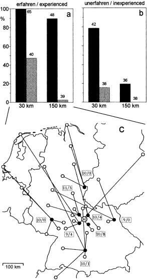
a, b: Heimkehrerfolg alter, stark erfahrener (a) und junger, unerfahrener (b) Brieftauben, gleichzeitig aufgelassen an je 4 symmetrisch um den Heimatort Würzburg gelegenen Orten in 30 bzw. 150 km Entfernung. Schwarz: unbehandelte Kontrollvögel, kreuzschraffiert: anosmische Vögel mit beidseitig durchtrennten Geruchsnerven. An den verwendeten Auflassplätzen waren auch die erfahrenen Tauben vorher noch nicht aufgelassen worden. Zahlen = Anzahl aufgelassener Tauben. c: Wiederfunde alt-erfahrener anosmischer Tauben von den 8 durch schwarze Punkte markierten Auflassplätzen; H = Heimatort. Umrahmte Zahlen: Anzahl aufgelassen/heimgekehrt (nach Wallraff et al. 1989). Fig. 3. a, b: Return rates of old, very experienced (a) and young, inexperienced (b) homing pigeons, simultaneously released at 4 sites symmetrically distributed around their home near Würzburg at distances of 30 and 150 km respectively. Filled columns: control birds, cross-hatched: anosmic birds with bilateral olfactory nerve section. The experienced pigeons had not previously been released at the sites used now, but were more or less familiar with a larger area around home. Numbers = number of birds released. c: Recoveries of old experienced anosmic pigeons from the 8 release sites as marked by filled circles; H = home site. Numbers in frames: birds released/returned.

Figure Abb. 5. 

Open in figure viewerPowerPoint

Luft-Filterung. Bis kurz vor dem Abflug saßen die Tauben in einem luftdichten Kasten, durch den natürliche Außenluft gesaugt wurde (links) oder durch Aktivkohle gefilterte Luft (rechts). Sofort nach He­rausnahme aus dem Kasten, einige Minuten vor dem Abflug, wurden die Riechepithelien jeder Taube durch einen Xylocain-Spray anästhetisiert. Gezeigt ist eine Zusammenfassung der Verschwinderichtungen von 46 Auflassungen, paarweise aus entgegengesetzten Richtungen bei gleicher Entfernung mit Vögeln gleicher oder ähnlicher Erfahrung (je n = 434 Abflüge; 2 Heimatschläge in Deutschland, 2 in Italien). Die Pfeile symbolisieren die mittleren Vektoren pro Auflassung (vgl. Abb. 2). Das Gesamtmittel (in Zahlen: Richtung, Vektor-Länge und -Heimkomponente) aus je 46 Vektoren entspricht dem Zentrum der kleinen Ellipsen, die die Konfidenzbereiche 95 % und 99 % angeben. Der P-Wert steht für die Differenz zwischen den Heimkomponenten pro Auflassung (Daten von Wallraff & Foà 1981, ergänzt durch weitere). Fig. 5. Air filtration. Until shortly before release, the pigeons were sitting in an airtight container ventilated with either natural environmental air (left) or with air sucked through a filter made of activated charcoal (right). Immediately after removal from the container, the olfactory epithelia of each pigeon (experimentals as well as controls) were anaesthetized by a spray of xylocain. Diagrams show vanishing bearings of 46 releases pooled, which were conducted pairwise from opposing directions and similar distances with birds of equal or similar experience (n = 434 bearings per diagram; 2 home lofts in Germany, 2 in Italy). The arrows symbolise the mean vectors per release (cf. Fig. 2). The overall mean (in numbers: direction, length and homeward component of vector) from 46 single-release vectors corresponds to the centre of the small ellipses which indicate the 95 % and 99 % confidence intervals. P refers to differences between homeward components per release.

Figure Abb. 6. 

Open in figure viewerPowerPoint

Orts-Simulation. Links: In Filterkästen (vgl. Abb. 5) wurde je eine Taubengruppe zu einander etwa gegenüber liegenden Orten A und B gebracht. Dort konnten sie gleichzeitig 3 h lang Naturluft riechen, danach wieder nur gefilterte Luft. Anschließend wurden die Tauben vom Ort B nach A gebracht (links) bzw. von A nach B (rechts). Dort wurden die Vögel beider Gruppen unter Nasalanästhesie abwechselnd freigelassen. Die Verschwinderichtungen der Kontrolltauben (Naturluft-Exposition am Auflassort) sind schwarz markiert, die der Experimentaltauben (Naturluft-Exposition am gegenüber liegenden Ort, Heimrichtung von dort siehe Außenpfeil) weiß. – Rechts: Summenprozentkurven der Heimkehrleistungen von allen 10 derartigen Versuchen zusammengefasst. Schwarze und weiße Symbole wie links. Die Kurve ohne Symbole stammt von einer dritten Taubengruppe, die den Umweg der „weißen” Gruppe mitgemacht hat, aber durchweg nur gefilterte Luft atmen konnte (nach Benvenuti & Wallraff 1985). Fig. 6. Site simulation. Left: At the same time, one filter box (cf. Fig. 5) with pigeons was brought to site A, another one to a roughly opposing site B. Over a simultaneous period of 3 h, the birds were permitted to smell natural air at these sites. Afterwards the charcoal filters were reinstalled and remained in position until release. Pigeons from site B were transported to site A (left), or those from A to B (right), where the others remained waiting. Birds of each group were alternately released under nasal anaesthesia. Vanishing bearings and resulting mean vectors of controls (exposure to natural air at the release site) are marked by filled symbols, those of experimentals (exposure to natural air at the opposite site; homeward direction from there see peripheral arrow) by empty symbols. – Right: Cumulative percentage curves of homing performance of all 10 such experiments pooled. Filled and empty symbols as on the left. The curve without symbols refers to a third group of pigeons which made the detour together with the „white” group, but inhaled filtered air all the time.

Figure Abb. 7. 

Open in figure viewerPowerPoint

Wind-Manipulation. a: Die Tauben lebten am Heimatort in einer Voliere, in welcher der ankommende Wind nach links, nicht oder nach rechts abgelenkt war (Beispiele für Südwind). Die Diagramme (Heimrichtung oben) zeigen die zugeordneten Verschwinderichtungen an drei verschiedenen Orten (durch Symbole unterschieden). Die Pfeile geben den mittleren Vektor (vgl. Abb. 2) aus den je 3 Einzelvektoren wieder (nach Baldaccini et al. 1975). – b: Die Tauben waren in korridorartigen Volieren künstlichem Wind ausgesetzt, der durch große Ventilatoren erzeugt wurde und in seiner Richtung in etwa dem jeweiligen Naturwind entsprach (schwarze Symbole) oder diesem entgegengesetzt war (weiße Symbole) (bei Wind von Osten waren die hier still gezeigten Ventilatoren aktiviert). Die entsprechend symbolisierten Abflugrichtungen sind für zwei Versuche gezeigt, denen die in weiteren Versuchen ähnelten (nach Ioalè et al. 1978). Fig. 7. Manipulation of winds. a: At the home site, some of the pigeons lived in an aviary in which the wind was deflected either to the left or to the right (examples showing wind from south). The diagrams (home upwards) show corresponding vanishing bearings at three different sites as distinguished by symbols. Arrows indicate mean vectors calculated from 3 single-release vectors. – b: At the home site, pigeons lived in corridor-shaped aviaries in which they were exposed to winds produced by a large ventilator. Wind direction either corresponded, by and large, to the current natural wind (filled symbols) or was opposite to it (empty symbols) (with wind from the east, the ventilators were activated that are shown here as still). The corresponding initial bearings of two representative releases are shown as examples.

Figure Abb. 8. 

Open in figure viewerPowerPoint

Relief-Darstellung des standardisierten proportionalen Anteils von 6 Kohlenwasserstoff-Verbindungen an deren Gesamtmenge in der bodennahen Atmosphäre eines Gebiets von 300 × 300 km um Würzburg als Zentrum. Gegenden, in denen der relative Anteil der betreffenden Substanz über ihrem Gesamtmittel lag, sind hell gezeichnet, solche mit unterdurchschnittlichem Anteil dunkel. Die kleinen Diagramme zeigen Mittelwerte in Distanzklassen entlang dem errechneten Gradienten, dessen Aufwärts-Richtung angegeben ist (Ordinate = Differenz vom Gesamtmittel in Einheiten der Standardabweichung) (aus Wallraff & Andreae 2000). Fig. 8. Relief maps showing standardised ratios of six hydrocarbons, relative to the sum of all six, in the ground-level atmosphere of an area of 300 × 300 km centred at Würzburg, Germany. Regions in which the relative portion of the respective compound was above its overall mean are shown bright, those with ratios below average dark. Small diagrams show means in classes of distance along the computed gradient whose upwards direction is indicated (ordinate = difference from overall mean in units of standard deviation).

Figure Abb. 9. 

Open in figure viewerPowerPoint

Aus den in Abb. 8 gegebenen Daten errechnete „Abflugrichtungen” an 12 Orten in 150 km Entfernung rings um Würzburg. Aus der Kenntnis der Gradientenrichtungen und aus den am Ort gemessenen skalaren Werten als Differenz zum Gesamtmittel ergeben sich je 6 Einzelvektoren, die zu einem resultierenden Vektor (Pfeil) kombiniert werden (aus Wallraff 2000a). Fig. 9. Computed „initial bearings” at 12 sites 150 km distant from Würzburg, deduced from the atmospheric data shown in Fig. 8. From knowledge of gradient directions (which birds hypothetically determine at the home site by correlating winds with odours) and local measurement of 6 ratios as differences from their overall means, 6 individual vectors were calculated and combined to a resulting vector (arrow), whose length may correspond to the degree of angular scatter in a sample of real ­pigeons.

Figure Abb. 10. 

Open in figure viewerPowerPoint

Heimkehrerfolg von Staren, die über verschiedene Entfernungen nach Osten oder Westen von ihrem Brutplatz in Oberbayern verfrachtet wurden. Säulen (linke Ordinate): Prozentsatz der Heimkehrer; kreuzschraffiert: durch bilaterale Nervdurchtrennung anosmisch gemachte Vögel, schwarz: scheinoperierte Kontrollvögel. Mit Linien verbundene Punkte (rechte Ordinate): Heimkehrrate der anosmischen Stare im Verhältnis zur Rate der Kontrollen (jeweilige schwarze Säule = 100 %). Die Zahlen geben die Anzahlen der verfrachteten Stare (nach Wallraff et al. 1995). Fig. 10. Homing success of starlings displaced over varying distances east or west from their breeding site in southern Bavaria. Columns (left ordinate): percentage of birds returned over birds released; crosshatched: starlings made anosmic by bilateral nerve section, black: sham-operated control birds. Line-connected dots (right ordinate): Return rate of anosmic starlings as a percentage of the rate of controls (respective black column = 100 %). Numbers give sample sizes of displaced starlings.

Figure Abb. 11. 

Open in figure viewerPowerPoint

Prozentsätze der nach dem Zug im folgenden Frühjahr an den kontrollierten Nistkästen wieder beobachteten Stare. OLF = olfaktorisch intakte, ANO = anosmische Vögel (nach Wallraff et al. 1995). Fig. 11. Percentage of starlings re-observed at the breeding site after migration in the following spring. OLF = olfactorily intact control birds, ANO = anosmic birds.

Figure Abb. 12. 

Open in figure viewerPowerPoint

Schema zur hypothetischen Rolle der olfaktorischen Navigation beim Weitstrecken-Zug. Das als visuell bekannt angenommene Gebiet ist schwarz, der olfaktorisch beherrschbare Navigationsbereich grau markiert. Der gestrichelte Strahl gibt die genetisch programmierte Kompassrichtung wieder, die vom Vogel (dicke Pfeile) aktiv eingehalten wird, von der er aber durch Seitenwinde verdriftet bzw. durch eine ökologische Barriere (gepunktet) abgelenkt wird. a: erster Herbstzug, b: Frühjahrszug. Weiteres im Text. Fig. 12. Scheme explaining the hypothetical role of olfactory navigation in long-distance migration. The area thought to be visually familiar is black, the range within which olfactory navigation is thought possible is grey. The dashed line with arrowhead indicates the genetically programmed compass direction, which is actively intended by the bird (thick arrows), but from which it is deflected by side winds or an ecological barrier (dotted area). a: first autumn migration, b: spring migration. In a, the bird reaches, by following its population-specific time-and-direction programme, a roughly determined wintering region within which it looks for an ecologically suitable habitat. In b, to reach directly the small familiar breeding area, the bird would have to stay within a very narrow angular range (thin dashed arrow rays). This is impossible, and it is unnecessary, if the bird only needs to reach a much larger target area within which it is able to home by using olfactory gradients.

Figure Abb. 13. 

Open in figure viewerPowerPoint

a–c: Durch Satellitentelemetrie beobachtete spontane Exkursionen dreier Wander-Albatrosse (Diomedea exulans) über dem südwestlichen Indischen Ozean (a, b: nach Jouventin & Weimerskirch 1990 aus Papi & Luschi 1996) bzw. dem südlichen Atlantik (c: nach Prince et al. 1992). Die Start- und Ziel-Heimatinsel ist durch einen Kreis markiert. Die Punkte auf der Route kennzeichnen die einzelnen Lokalisationen (in c: schwarz = Nacht, weiß = Tag). Die Entfernungsskalen sind (wegen der Projektionsverzerrungen) approximativ. – d: Heimkehrversuche mit Laysan-Albatrossen (Diomedea immutabilis), die vom Midway-Atoll (Nordpazifik) aus in verschiedene Richtungen verfrachtet wurden. Angegeben sind die Entfernungen sowie die Anzahl der verfrachteten / zurückgekehrten Vögel und die Dauer bis zur Wiederbeobachtung auf der Heimatinsel (nach Daten von Kenyon & Rice 1958, verändert aus Papi & Wallraff 1992). Fig. 13. a–c: Spontaneous excursions of three wandering albatrosses observed by satellite telemetry over the south-western Indian Ocean (a, b) and the southern Atlantic (c) respectively. The home island is marked by a circle. Dots along the route indicate localisations (in c: filled = night time, open = daytime). Distance scales are approximate (owing to map distortions by projection). – d: Homing experiments with Laysan albatrosses that were displaced in various directions from the Midway Atoll (northern Pacific). Indicated are distances as well as displaced/returned birds and the duration until re-observation on the home island.

Figure Abb. 14. 

Open in figure viewerPowerPoint

Konzentrationen zweier atmosphärischer Spurengase, vom Schiff aus gemessen über dem Atlantik während derselben Fahrt im Oktober/November 1996 etwa entlang dem Meridian 30 °W von Nord nach Süd (Daten von Weller et al. 2000 und Fischer et al. 2000). Fig. 14. Concentrations of two atmospheric trace gases measured on board a ship over the Atlantic Ocean during the same cruise in October/November 1996 roughly along the meridian 30 °W from north to south.